![]()
![]()

Personalized luminous exposure data is progressively gaining importance in various sectors, including research, occupational affairs, and fitness tracking. Data are collected through a proliferating selection of wearable loggers and dosimeters, varying in size, shape, functionality, and output format. Despite or maybe because of numerous use cases, the field lacks a unified framework for collecting, validating, and analyzing the accumulated data. This issue increases the time and expertise necessary to handle such data and also compromises the FAIRness (Findability, Accessibility, Interoperability, Reusability) of the results, especially in meta-analyses.
LightLogR is a package under development as part of the MeLiDos project to address these issues. The package aims to provide tools for:
Import from common measurement devices (see below for a list of Supported devices)
Cleaning and processing of light logging data
Visualization of light exposure data, both exploratory and publication ready
Calculation of common analysis parameters (see below for a list of Metrics)
To come:
Import, creation, and verification of crucial metadata
Semi-automated analysis and visualization (both command-line and GUI-based)
Integration of data into a unified database for cross-study analyses
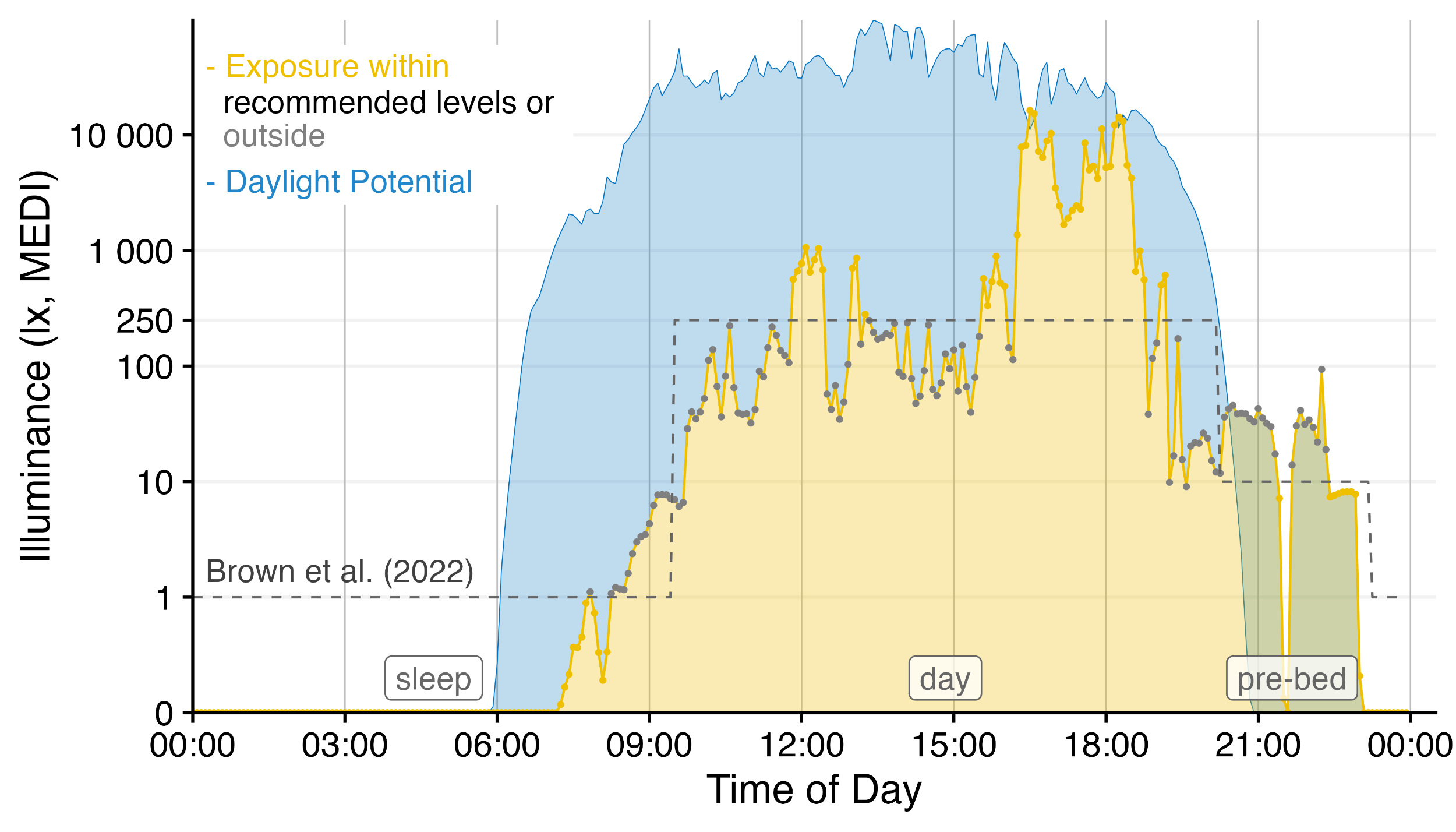
Have a look at the Example section down below to get started, or dive into the Articles to get more in depth information about how to work with the package and generate images such as the one above, import data, visualization, and metric calculation.
You can install LightLogR from CRAN with:
install.packages("LightLogR")You can install the latest development version of LightLogR from GitHub with:
# install.packages("devtools")
devtools::install_github("tscnlab/LightLogR")Here is a quick starter on how to use LightLogR.
library(LightLogR)
#the following packages are needed for the examples as shown below.
library(flextable)
library(dplyr)
#> Warning: package 'dplyr' was built under R version 4.5.2
library(ggplot2)
#> Warning: package 'ggplot2' was built under R version 4.5.2You can import a light logger dataset with ease. The import functions give quick, helpful feedback about the dataset.
filename <-
  system.file("extdata/205_actlumus_Log_1020_20230904101707532.txt.zip",
              package = "LightLogR")
dataset <- import$ActLumus(filename, "Europe/Berlin", manual.id = "P1")
#>
#> Successfully read in 61'016 observations across 1 Ids from 1 ActLumus-file(s).
#> Timezone set is Europe/Berlin.
#> The system timezone is Europe/Madrid. Please correct if necessary!
#>
#> First Observation: 2023-08-28 08:47:54
#> Last Observation: 2023-09-04 10:17:04
#> Timespan: 7.1 days
#>
#> Observation intervals:
#>   Id    interval.time     n pct
#> 1 P1    10s           61015 100%
For more complex data, there is the useful gg_overview()
function to get an immediate grasp of your data. It was automatically
called during import (set auto.plot = FALSE to suppress
this), but really shines for datasets with multiple participants. It
also indicates where data is missing, based on the measurement epochs
found in the data.
note: the above example image requires a large dataset, not included in the package. It is available, however, in the article on Import & cleaning.
#example code, on how to use gg_overview():
dataset %>% gg_overview()Once imported, LightLogR has many convenient visualization options.
dataset %>% gg_days()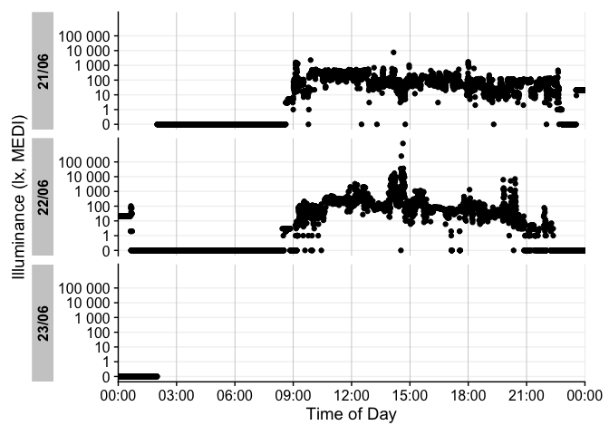
There is a wide range of options to the gg_days()
function to customize the output. Have a look at the reference page
(?gg_days) to see all options. You can also override most
of the defaults, e.g., for different color,
facetting, theme options. Helper functions can
prepare the data (e.g. to aggregate it to coarser intervals), or to add
to the plot (e.g., to add conditions, such as nighttime)
dataset |>
  #change the interval from 10 seconds to 15 minutes:
  aggregate_Datetime("15 min") |>
  #create groups of 3-hour intervals:
  cut_Datetime("3 hours") |>
  #plot creation, with a boxplot:
  gg_days(geom = "boxplot", group = Datetime.rounded) |>
  #adding nighttime indicators:
  gg_photoperiod(c(47.9,9)) +
  # the output is a standard ggplot, and can be manipulated that way
  geom_line(col = "red", linewidth = 0.25) +
  labs(title = "Personal light exposure across a week",
       subtitle = "Boxplot in 3-hour bins")
#> Warning: Orientation is not uniquely specified when both the x and y aesthetics are
#> continuous. Picking default orientation 'x'.
#> Orientation is not uniquely specified when both the x and y aesthetics are
#> continuous. Picking default orientation 'x'.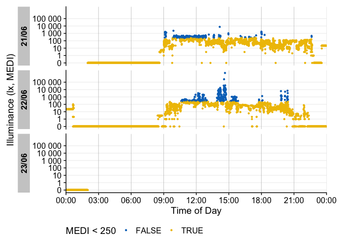
The built-in dataset sample.data.environment shows a
combined dataset of light logger data and a second set of data - in this
case unobstructed outdoor light measurements. Combined datasets can be
easily visualized with gg_day(). The col
parameter used on the Id column of the dataset allows for a
color separation.
sample.data.environment %>%
  gg_day(
    start.date = "2023-09-01",
    aes_col = Id,
    geom = "line") +
  theme(legend.position = "bottom")
#> Only Dates will be used from start.date and end.date input. If you also want to set Datetimes or Times, consider using the `filter_Datetime()` function instead.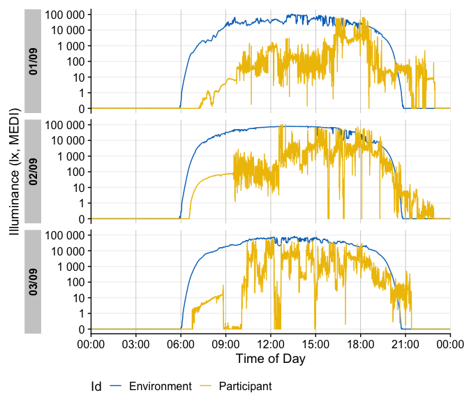
gg_day() will show plots always facetted by day, whereas
gg_days() shows a timeline of days for each group. Both
functions are opinionated in terms of the scaling and linebreaks to only
show whole days, all of which can be adjusted.
There are many ways to enhance the plots - if, e.g., we look for periods of at least 1 hour above 250 lx, we can add and then visualize these periods easily
sample.data.environment %>%
  #search for these conditions:
  add_clusters(MEDI > 250, cluster.duration = "30 min") |>
  #base plot + add the condition
  gg_days() |>
  gg_states(state, fill = "red") +
  #standard ggplot:
  geom_hline(yintercept = 250, col = "red", linetype = "dashed") +
  labs(title = "Periods > 250 lx mel EDI for more than 30 minutes")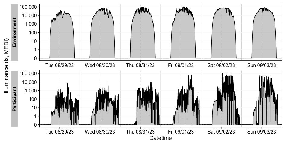
There are more visualizations to try - the article on Visualizations dives into them in-depths.
sample.data.environment |> gg_heatmap(doubleplot = "next")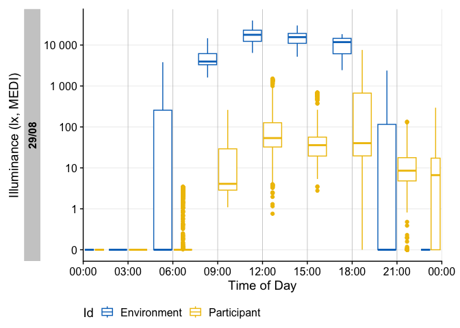
There are many Metrics used in literature for
condensing personalized light exposure time series to singular values.
LightLogR has a rather comprehensive number of these
metrics with a consistent, easy-to-use interface.
sample.data.environment |> # two groups: participant and environment
  filter_Date(length = "2 days") |> #filter to three days each for better overview
  group_by(Day = lubridate::date(Datetime), .add = TRUE) |>  #add grouping per day
  summarize(
    #time above 250 lx mel EDI:
    duration_above_threshold(MEDI, Datetime, threshold = 250, as.df = TRUE),
    #intradaily variability (IV):
    intradaily_variability(MEDI, Datetime, as.df = TRUE),
    #... as many more metrics as are desired
    .groups = "drop"
  )
#> # A tibble: 4 × 4
#>   Id          Day        duration_above_250    intradaily_variability
#>   <fct>       <date>     <Duration>                             <dbl>
#> 1 Environment 2023-08-29 48240s (~13.4 hours)                   0.248
#> 2 Environment 2023-08-30 49350s (~13.71 hours)                  0.168
#> 3 Participant 2023-08-29 5810s (~1.61 hours)                    1.23
#> 4 Participant 2023-08-30 9960s (~2.77 hours)                    0.821
Other types of metrics can be derived less formally by the
durations(), extract_state() or
extract_cluster() function.
dataset |>
  gap_handler(full.days = TRUE) |> #extend the viewed time until midnight of the first and last day
  durations(MEDI, show.missing = TRUE)
#> # A tibble: 1 × 4
#> # Groups:   Id [1]
#>   Id    duration              missing               total
#>   <fct> <Duration>            <Duration>            <Duration>
#> 1 P1    610160s (~1.01 weeks) 81040s (~22.51 hours) 691200s (~1.14 weeks)

dataset |>
  group_by(TAT250 = MEDI >= 250, .add = TRUE) |> #creating a grouping column that checks for values above 250lx
  durations(MEDI)
#> # A tibble: 2 × 3
#> # Groups:   Id, TAT250 [2]
#>   Id    TAT250 duration
#>   <fct> <lgl>  <Duration>
#> 1 P1    FALSE  498530s (~5.77 days)
#> 2 P1    TRUE   111630s (~1.29 days)
The second row indicates where this status is true. This will be identical to:
dataset |>
  summarize(
    duration_above_threshold(MEDI, Datetime, threshold = 250, as.df = TRUE),
    .groups = "drop"
  )
#> # A tibble: 1 × 2
#>   Id    duration_above_250
#>   <fct> <Duration>
#> 1 P1    111630s (~1.29 days)
What if we are interested in how often this threshold is crossed, and for how long?
dataset |>
  extract_states(TAT250, MEDI >= 250) |> #extract a list of states
  summarize_numeric() |> #summarize the numeric values
  select(Id, TAT250, mean_duration, episodes, total_duration) #collect a subset
#> # A tibble: 2 × 5
#> # Groups:   Id [1]
#>   Id    TAT250 mean_duration        episodes total_duration
#>   <fct> <lgl>  <Duration>              <int> <Duration>
#> 1 P1    FALSE  482s (~8.03 minutes)     1034 498530s (~5.77 days)
#> 2 P1    TRUE   108s (~1.8 minutes)      1034 111630s (~1.29 days)
We see that there are roughly one thousand instances across the week where 250 lx was reached, but it only lasted under two minutes on average. How many long periods are there, say above 30 minutes? As there might be short interruption, that we consider irrelevant, we are ignoring interruptions of 1 minute. This is the area of clusters.
dataset |>
  extract_clusters(MEDI >= 250, #base condition
                   cluster.duration = "30 mins", #search for at least 30 minute instances
                   interruption.duration = "1 min", #allow 1 minute interrupts
                   add.label = TRUE) |> #add a description of the conditions
  group_by(label) |> #group by the label so it does not get removed next
  summarize_numeric() |> #summarize the output
  select(-mean_epoch) #collect a subset
#> # A tibble: 1 × 6
#>   label   mean_start mean_end mean_duration       total_duration        episodes
#>   <chr>   <time>     <time>   <Duration>          <Duration>               <int>
#> 1 MEDI>=… 13:50:47   15:02:14 4288s (~1.19 hours) 72890s (~20.25 hours)       17
We see there are only 17 instances across the week, lasting, on average, a bit above an hour (and sitting aroung 14:00 - 15:00). Directly relating the total duration to the 1.29 days time above 250 lx from above would be misleading, however. This is because here, there are interruptions present. How prominent are these interruptions?
dataset |>
  extract_clusters(MEDI >= 250, #base condition
                   cluster.duration = "30 mins", #search for at least 30 minute instances
                   interruption.duration = "1 min", #allow 1 minute interrupts
                   add.label = TRUE) |>
  #extract the metric:
  extract_metric(dataset, rel_interrupt = sum(MEDI < 250)/n()) |>
  summarize_numeric(prefix = "") |> #summarize the output
  select(episodes, total_duration, rel_interrupt) |>   #collect a subset
  mutate(interrupt_duration = (total_duration*rel_interrupt) |> round(), #calculate interrupt
         rel_interrupt = rel_interrupt |> scales::percent_format(1)())
#> # A tibble: 1 × 4
#>   episodes total_duration        rel_interrupt interrupt_duration
#>      <int> <Duration>            <chr>         <Duration>
#> 1       17 72890s (~20.25 hours) 4%            2918s (~48.63 minutes)
Thus we find that only about 4% of the long exposure periods are made up of interruptions, or just shy of 50 minutes out of over 20 hours.
LightLogR provides a range of functions to get insight into your light logger data. Most importantly, you can search for and eliminate implicit gaps.
sample.data.irregular |> has_irregulars()
#> [1] TRUE
sample.data.irregular |> has_gaps()
#> [1] TRUE
At import, we already get a sense for intervals, but can always show
them with count_difftime().
sample.data.irregular %>% count_difftime()
#> # A tibble: 4 × 4
#> # Groups:   Id [1]
#>   Id    difftime       n group.indices
#>   <chr> <Duration> <int>         <int>
#> 1 P1    15s        10015             1
#> 2 P1    16s         1367             1
#> 3 P1    17s           23             1
#> 4 P1    18s           16             1
We can eliminate this through the gap_handler()
function. This function will automatically fill in the gaps with NA
values. The function will not impute or interpolate
data. As the most dominant interval in the dataset is now not
15 seconds anymore (because intermediate datapoints have been added), we
need to specify the epoch for gap_finder().
sample.data.irregular |> gap_handler() |> has_gaps(epoch = "15 secs")
#> [1] FALSE
If we want to force the data to be regular, we can use the
aggregate_Datetime() function. This will aggregate the data
to the specified epoch. There are sensible defaults on how to aggregate
numeric, categorical, and logical data. You can also specify your own
aggregation functions.
sample.data.irregular |>
  aggregate_Datetime(unit = "20 sec") |>
  has_gaps()
#> [1] FALSE
There are also convenient functions to extract
(extract_gaps()), summarize (gap_table()) or
visualize (gg_gaps()) gaps.
dataset |> gg_gaps()
#> Warning: Removed 8104 rows containing missing values or values outside the scale range
#> (`geom_line()`).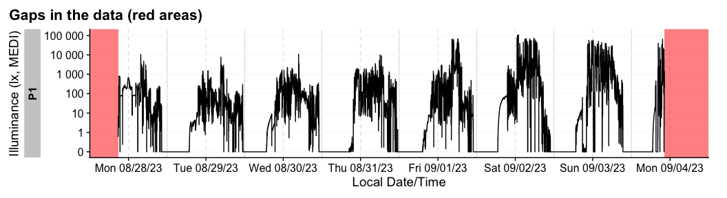
Finally, the remove_partial_data() easily gets rid of
groups or days that do not provide enough data.
dataset |>
  remove_partial_data(MEDI, #variable for which to check missingness
                      threshold.missing = "2 hours", #remove when more than 2 hours are missing
                      by.date = TRUE, #check the condition per day, not the whole participant
                      handle.gaps = TRUE) |>  #go beyond the available data to midnight of the first and last day
  gg_days()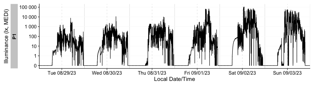
At present, these are the devices we support in LightLogR:
Actiwatch_Spectrum
ActLumus
ActTrust
Circadian_Eye
Clouclip
DeLux
GENEActiv_GGIR
Kronowise
LiDo
LightWatcher
LIMO
LYS
MiEye
MotionWatch8
nanoLambda
OcuWEAR
Speccy
SpectraWear
VEET
More Information on these devices can be found in the reference for
import_Dataset(). If you want to know how to import data
from these devices, have a look at our article on Import
& Cleaning.
If you are using a device that is currently not supported, please contact the developers. We are always looking to expand the range of supported devices. The easiest and most trackable way to get in contact is by opening a new issue on our Github repository. Please also provide a sample file of your data, so we can test the import function.
LightLogR supports a wide range of metrics across different metric families. You can find the full documentation of metrics functions in the reference section. There is also an overview article on how to use Metrics.
| Metric Family | Submetrics | Note | Documentation |
|---|---|---|---|
| Barroso | 7 | barroso_lighting_metrics() |
|
| Bright-dark period | 4x2 | bright / dark | bright_dark_period() |
| Centroid of light exposure | 1 | centroidLE() |
|
| Dose | 1 | dose() |
|
| Disparity index | 1 | disparity_index() |
|
| Duration above threshold | 3 | above, below, within | duration_above_threshold() |
| Exponential moving average (EMA) | 1 | exponential_moving_average() |
|
| Frequency crossing threshold | 1 | frequency_crossing_threshold() |
|
| Intradaily Variance (IV) | 1 | intradaily_variability() |
|
| Interdaily Stability (IS) | 1 | interdaily_stability() |
|
| Midpoint CE (Cumulative Exposure) | 1 | midpointCE() |
|
| nvRC (Non-visual circadian response) | 4 | nvRC(), nvRC_circadianDisturbance(),
nvRC_circadianBias(),
nvRC_relativeAmplitudeError() |
|
| nvRD (Non-visual direct response) | 2 | nvRD(), nvRD_cumulative_response() |
|
| Period above threshold | 3 | above, below, within | period_above_threshold() |
| Pulses above threshold | 7x3 | above, below, within | pulses_above_threshold() |
| Threshold for duration | 2 | above, below | threshold_for_duration() |
| Timing above threshold | 3 | above, below, within | timing_above_threshold() |
| Total: | |||
| 17 families | 62 metrics |
If you would like to use a metric you don’t find represented in LightLogR, please contact the developers. The easiest and most trackable way to get in contact is by opening a new issue on our Github repository.
LightLogR is developed by the Translational Sensory & Circadian Neuroscience Unit (MPS/TUM/TUMCREATE, a joint group based at the Max Planck Institute for Biological Cybernetics, the Technical University of Munich, and TUMCREATE, .
MeLiDos is a joint, EURAMET-funded project involving sixteen partners across Europe, aimed at developing a metrology and a standard workflow for wearable light logger data and optical radiation dosimeters. Its primary contributions towards fostering FAIR data include the development of a common file format, robust metadata descriptors, and an accompanying open-source software ecosystem.
![]()

The project (22NRM05 MeLiDos) has received funding from the European Partnership on Metrology, co-financed from the European Union’s Horizon Europe Research and Innovation Programme and by the Participating States. Views and opinions expressed are however those of the author(s) only and do not necessarily reflect those of the European Union or EURAMET. Neither the European Union nor the granting authority can be held responsible for them.
LightLogR is further supported throught the Wellcome trust and the GLEE project (Global Light exposure engine).
![]()
![]()
All types of contributions are encouraged and valued. See the CONTRIBUTING section for different ways to help and details about how this project handles them. This project and everyone participating in it is governed by the LightLogR Code of Conduct.