![]()
![]()
![]()
Unobservable group structures are a common challenge in panel data analysis. Disregarding group-level heterogeneity can introduce bias. Conversely, estimating individual coefficients for each cross-sectional unit is inefficient and may lead to high uncertainty. Furthermore, neglecting time-variance in slope coefficients can lead to inconsistent and misleading results, even in large panels.
This package efficiently addresses these issues by implementing the pairwise adaptive group fused Lasso (PAGFL) by Mehrabani (2023) and FUSE-TIME–Fused Unobserved group Spline Estimation–by Haimerl et al. (2025). PAGFL is a regularizer that identifies latent group structures and estimates group-specific coefficients in a single step. FUSE-TIME generalizes this to smoothly time-varying coefficients.
The PAGFL package makes these powerful procedures easy
to use.
Always stay up-to-date with the development version (1.1.4) of
PAGFL from GitHub:
# install.packages("devtools")
devtools::install_github("Paul-Haimerl/PAGFL")
library(PAGFL)
The stable version (1.1.4) is available on CRAN:
install.packages("PAGFL")The PAGFL package includes a function that automatically
simulates a panel data set with a group structure in the slope
coefficients:
# Simulate a simple panel with three distinct groups and two exogenous explanatory variables
set.seed(1)
sim <- sim_DGP(N = 20, n_periods = 150, p = 2, n_groups = 3)
data <- sim$data
\[y_{it} = \beta_i^{0 \prime} x_{it} + \gamma_i + u_{it}, \quad i = 1, \dots, N, \quad t = 1, \dots, T,\]
where \(y_{it}\) is a scalar dependent variable, \(x_{it}\) a \(p \times 1\) vector of explanatory variables, and \(\gamma_i\) reflects an individual fixed effect. The \(p\)-dimensional vector slope coefficients \(\beta_i^0\) follows the (latent) group structure
\[\beta_{i} = \sum_{k = 1}^K \alpha_k 1 \{i \in G_k \},\]
with \(\cup_{k = 1}^K G_k = \{1, \dots, N \}\), and \(G_k \cap G_j = \emptyset\) as well as \(\| \alpha_k \neq \alpha_j \|\) for any \(k \neq j\), \(k,j = 1, \dots, K\) (see Mehrabani 2023, sec. 2).
sim_DGP() also nests, among other, all DGPs employed in
the simulation study of Mehrabani (2023,
sec. 6).
To execute the PAGFL procedure, pass the dependent and independent variables, the number of time periods, and a penalization parameter \(\lambda\).
estim <- pagfl(y ~ ., data = data, n_periods = 150, lambda = 20, verbose = F)
summary(estim)
#> Call:
#> pagfl(formula = y ~ ., data = data, n_periods = 150, lambda = 20,
#>     verbose = F)
#>
#> Balanced panel: N = 20, T = 150, obs = 3000
#>
#> Convergence reached:
#> TRUE (49 iterations)
#>
#> Information criterion:
#>     IC lambda
#>  1.354 20.000
#>
#> Residuals:
#>      Min       1Q   Median       3Q      Max
#> -4.47230 -0.72086 -0.00120  0.76214  4.31838
#>
#> 2 groups:
#>  1  2  3  4  5  6  7  8  9 10 11 12 13 14 15 16 17 18 19 20
#>  1  1  2  1  1  1  1  2  1  1  2  2  2  1  1  1  1  1  2  1
#>
#> Coefficients:
#>                X1       X2
#> Group 1 -0.36838  1.61275
#> Group 2 -0.49489 -1.23534
#>
#> Residual standard error: 1.15012 on 2978 degrees of freedom
#> Mean squared error: 1.31307
#> Multiple R-squared: 0.65845, Adjusted R-squared: 0.65605
pagfl() returns an object of type pagfl,
which holds
model: A data.frame containing the
dependent and explanatory variables as well as individual and time
indices (if provided).coefficients: A \(K \times
p\) matrix of the post-Lasso group-specific parameter
estimates.groups: A list containing (i) the total
number of groups \(\hat{K}\) and (ii) a
vector of estimated group memberships \((\hat{g}_1, \dots, \hat{g}_N)\), where
\(\hat{g}_i = k\) if \(i\) is assigned to group \(k\).residuals: A vector of residuals of the demeaned
model.fitted: A vector of fitted values of the demeaned
model.args: A list of additional arguments.IC: A list containing (i) the value of the
IC, (ii) the employed tuning parameter \(\lambda\), and (iii) the mean squared
error.convergence: A list containing (i) a
logical variable if convergence was achieved and (ii) the number of
executed ADMM algorithm iterations.call: The function call.[!TIP]
pagflobjects support a variety of useful generic functions likesummary(),fitted(),resid(),df.residual,formula, andcoef().
estim_fit <- fitted(estim)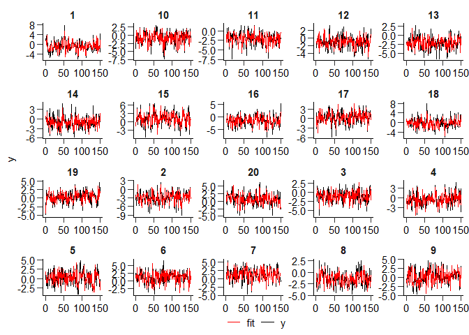
[!IMPORTANT] Selecting a \(\lambda\) value a priori can be tricky. For instance, it seems like
lambda = 20is too high since the number of groups \(K\) is underestimated.
We suggest iterating over a comprehensive range of candidate values to trace out the correct model. To specify a suitable grid, create a logarithmic sequence ranging from a penalty parameter that induces complete slope heterogeneity to complete slope homogeneity (i.e., \(\widehat{K} = 1\)). The resulting \(\lambda\) grid vector can be passed in place of any specific value, and a BIC IC selects the best-fitting parameter.
Furthermore, it is also possible to supply a data.frame
with named variables and choose a specific formula that selects the
variables in that data.frame, just like in the base
lm() function. If the explanatory variables in
X are named, these names also appear in the output.
colnames(data)[-1] <- c("a", "b")

lambda_set <- exp(log(10) * seq(log10(1e-4), log10(10), length.out = 10))
estim_set <- pagfl(y ~ a + b, data = data, n_periods = 150, lambda = lambda_set, verbose = F)
summary(estim_set)
#> Call:
#> pagfl(formula = y ~ a + b, data = data, n_periods = 150, lambda = lambda_set,
#>     verbose = F)
#>
#> Balanced panel: N = 20, T = 150, obs = 3000
#>
#> Convergence reached:
#> TRUE (51 iterations)
#>
#> Information criterion:
#>      IC  lambda
#> 1.12877 0.21544
#>
#> Residuals:
#>      Min       1Q   Median       3Q      Max
#> -3.47858 -0.66283 -0.02688  0.72880  3.77812
#>
#> 3 groups:
#>  1  2  3  4  5  6  7  8  9 10 11 12 13 14 15 16 17 18 19 20
#>  1  1  2  3  1  3  3  2  3  3  2  2  2  1  1  1  3  1  2  3
#>
#> Coefficients:
#>                 a        b
#> Group 1 -0.95114  1.61719
#> Group 2 -0.49489 -1.23534
#> Group 3  0.24172  1.61613
#>
#> Residual standard error: 1.03695 on 2978 degrees of freedom
#> Mean squared error: 1.06738
#> Multiple R-squared: 0.72236, Adjusted R-squared: 0.7204
When, as above, the specific estimation method is left unspecified,
pagfl() defaults to penalized Least Squares (PLS)
method = 'PLS' (Mehrabani, 2023,
sec. 2.2). PLS is very efficient but requires weakly exogenous
regressors. However, even endogenous predictors can be accounted for by
employing a penalized Generalized Method of Moments (PGMM)
routine in combination with exogenous instruments \(Z\).
Specify a slightly more elaborate endogenous and dynamic panel data set and apply PGMM. When encountering a dynamic panel data set, we recommend using a Jackknife bias correction, as proposed by Dhaene and Jochmans (2015).
# Generate a panel where the predictors X correlate with the cross-sectional innovation,
# but can be instrumented with q = 2 variables in Z. Furthermore, include GARCH(1,1)
# innovations, and specific group sizes
sim_endo <- sim_DGP(
  N = 20, n_periods = 200, p = 2, n_groups = 3, group_proportions = c(0.3, 0.3, 0.4),
  error_spec = "GARCH", q = 2
)
data_endo <- sim_endo$data
Z <- sim_endo$Z

# Note that the method PGMM and the instrument matrix Z need to be passed
estim_endo <- pagfl(y ~ ., data = data_endo, n_periods = 200, lambda = 2, method = "PGMM", Z = Z, bias_correc = TRUE, max_iter = 50e3, verbose = FALSE)
summary(estim_endo)
#> Call:
#> pagfl(formula = y ~ ., data = data_endo, n_periods = 200, lambda = 2,
#>     method = "PGMM", Z = Z, bias_correc = TRUE, max_iter = 50000,
#>     verbose = FALSE)
#>
#> Balanced panel: N = 20, T = 200, obs = 3980
#>
#> Convergence reached:
#> TRUE (14632 iterations)
#>
#> Information criterion:
#>      IC  lambda
#> 1.97129 2.00000
#>
#> Residuals:
#>      Min       1Q   Median       3Q      Max
#> -4.87011 -0.90055  0.01193  0.90767  5.54203
#>
#> 3 groups:
#>  1  2  3  4  5  6  7  8  9 10 11 12 13 14 15 16 17 18 19 20
#>  1  2  3  3  3  2  2  3  1  3  2  2  1  1  2  1  3  1  3  3
#>
#> Coefficients:
#>                X1       X2
#> Group 1  0.55337 -1.22836
#> Group 2 -0.88484 -0.89231
#> Group 3  1.60547 -1.43718
#>
#> Residual standard error: 1.38812 on 3958 degrees of freedom
#> Mean squared error: 1.91621
#> Multiple R-squared: 0.87079, Adjusted R-squared: 0.8701
[!TIP]
pagfl()lets you select a minimum group size, adjust the efficiency vs. accuracy trade-off of the iterative estimation algorithm, and modify a list of further settings. Visit the documentation?pagfl()for more information.
The package also includes the functions sim_tv_DGP() and
fuse_time(), which generate and estimate grouped panel data
models with smoothly time-varying coefficients \(\beta_i (t/T)\). As detailed in Haimerl et
al. (2025), the
functional coefficients admit to the group structure
\[\beta_{i} (t/T) = \sum_{k = 1}^K \alpha_k (t/T) \mathbb{1} \{i \in G_k \}.\]
The time-varying coefficients are estimated using polynomial B-spline functions, yielding a penalized sieve estimator (PSE) (see Haimerl et al., 2025, sec. 2).
# Simulate a time-varying panel with a trend and a group pattern
N <- 20
n_periods <- 100
tv_sim <- sim_tv_DGP(N = N, n_periods = n_periods, sd_error = 1, intercept = TRUE, p = 1)
tv_data <- tv_sim$data

tv_estim <- fuse_time(y ~ 1, data = tv_data, n_periods = n_periods, lambda = 5, verbose = F)
summary(tv_estim)
#> Call:
#> fuse_time(formula = y ~ 1, data = tv_data, n_periods = n_periods,
#>     lambda = 5, verbose = F)
#>
#> Balanced panel: N = 20, T = 100, obs = 2000
#>
#> Convergence reached:
#> TRUE (212 iterations)
#>
#> Information criterion:
#>      IC  lambda
#> 0.16648 5.00000
#>
#> Residuals:
#>      Min       1Q   Median       3Q      Max
#> -3.57761 -0.68826  0.00820  0.70118  3.40708
#>
#> 3 groups:
#>  1  2  3  4  5  6  7  8  9 10 11 12 13 14 15 16 17 18 19 20
#>  1  1  1  2  2  2  1  3  3  3  2  2  3  1  3  1  2  3  2  3
#>
#> Residual standard error: 1.02901 on 1974 degrees of freedom
#> Mean squared error: 1.04509
#> Multiple R-squared: 0.74213, Adjusted R-squared: 0.73886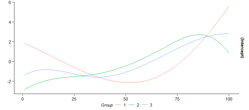
fuse_time() returns an object of class
fusetime, which contains
model: A data.frame containing the
dependent and explanatory variables as well as individual and time
indices (if provided).coefficients: A list holding (i) a \(T \times p^{(1)} \times \hat{K}\) array of
the post-Lasso group-specific functional coefficients and (ii) a \(K \times p^{(2)}\) matrix of time-constant
parameter estimates (when running a mixed time-varying panel data
model).groups: A list containing (i) the total
number of groups \(\hat{K}\) and (ii) a
vector of estimated group memberships \((\hat{g}_1, \dots, \hat{g}_N)\), where
\(\hat{g}_i = k\) if \(i\) is assigned to group \(k\).residuals: A vector of residuals of the demeaned
model.fitted: A vector of fitted values of the demeaned
model.args: A list of additional arguments.IC: A list containing (i) the value of the
IC, (ii) the employed tuning parameter \(\lambda\), and (iii) the mean squared
error.convergence: A list containing (i) a
logical variable if convergence was achieved and (ii) the number of
executed ADMM algorithm iterations.call: The function call.[!TIP] Again,
fusetimeobjects support genericsummary(),fitted(),resid(),df.residual,formula, andcoef()functions.
In empirical settings, unbalanced panel datasets are common; nevertheless, time-varying coefficient functions remain identifiable (see Haimerl et al. 2025, Appendix D). The spline functions simply interpolate missing time periods and the group structure compensates for missings in any individual cross-sectional unit. However, when using unbalanced datasets it is required to provide explicit indicator variables that declare the cross-sectional individual and time period each observation belongs to.
Lets delete 30% of observations, add indicator variables, and run
fuse_time() again.
# Draw some observations to be omitted
delete_index <- as.logical(rbinom(n = N * n_periods, prob = 0.7, size = 1))
# Construct cross-sectional and time indicator variables
tv_data$i_index <- rep(1:N, each = n_periods)
tv_data$t_index <- rep(1:n_periods, N)
# Delete some observations
tv_data <- tv_data[delete_index, ]
# Apply the time-varying PAGFL to an unbalanced panel
tv_estim_unbalanced <- fuse_time(y ~ 1, data = tv_data, index = c("i_index", "t_index"), lambda = 5, verbose = F)
summary(tv_estim_unbalanced)
#> Call:
#> fuse_time(formula = y ~ 1, data = tv_data, index = c("i_index",
#>     "t_index"), lambda = 5, verbose = F)
#>
#> Unbalanced panel: N = 20, T = 64-75, obs = 1379
#>
#> Convergence reached:
#> TRUE (950 iterations)
#>
#> Information criterion:
#>      IC  lambda
#> 0.18921 5.00000
#>
#> Residuals:
#>      Min       1Q   Median       3Q      Max
#> -3.43491 -0.69055 -0.00812  0.68488  3.63894
#>
#> 3 groups:
#>  1  2  3  4  5  6  7  8  9 10 11 12 13 14 15 16 17 18 19 20
#>  1  1  1  2  2  2  1  2  3  3  2  2  3  1  3  1  2  3  2  2
#>
#> Residual standard error: 1.04387 on 1353 degrees of freedom
#> Mean squared error: 1.06912
#> Multiple R-squared: 0.73683, Adjusted R-squared: 0.73197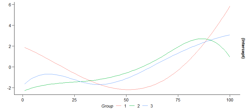
[!TIP]
fuse_time()lets you specify a lot more optionalities than shown here. For example, it is possible to adjust the polynomial degree and the number of interior knots in the spline basis system, or estimate a panel data model with a mix of time-varying and time-constant coefficients. See?fuse_time()for details.
It may occur that the group structure is known and does not need to
be estimated. In such instances, grouped_plm() and
grouped_tv_plm() make it easy to estimate a (time-varying)
linear panel data model given an observed grouping.
groups <- sim$groups
estim_oracle <- grouped_plm(y ~ ., data = data, n_periods = 150, groups = groups, method = "PLS")
summary(estim_oracle)
#> Call:
#> grouped_plm(formula = y ~ ., data = data, groups = groups, n_periods = 150,
#>     method = "PLS")
#>
#> Balanced panel: N = 20, T = 150, obs = 3000
#>
#> Information criterion: 1.12877
#>
#> Residuals:
#>      Min       1Q   Median       3Q      Max
#> -3.47858 -0.66283 -0.02688  0.72880  3.77812
#>
#> 3 groups:
#>  1  2  3  4  5  6  7  8  9 10 11 12 13 14 15 16 17 18 19 20
#>  1  1  2  3  1  3  3  2  3  3  2  2  2  1  1  1  3  1  2  3
#>
#> Coefficients:
#>                 a        b
#> Group 1 -0.95114  1.61719
#> Group 2 -0.49489 -1.23534
#> Group 3  0.24172  1.61613
#>
#> Residual standard error: 1.03695 on 2978 degrees of freedom
#> Mean squared error: 1.06738
#> Multiple R-squared: 0.72236, Adjusted R-squared: 0.7204
Besides not estimating the group structure,
grouped_plm() (grouped_tv_plm()) behave
identically to pagfl() (fuse_time())
The package is still under active development. Future versions are planned to include
You are not a R-user? Worry not - An equivalent Python library is in the works.
Feel free to reach out if you have any suggestions or questions.
Dhaene, G., & Jochmans, K. (2015). Split-panel jackknife estimation of fixed-effect models. The Review of Economic Studies, 82(3), 991-1030. DOI: doi.org/10.1093/restud/rdv007
Haimerl, P., Smeekes, S., & Wilms, I. (2025). Estimation of latent group structures in time-varying panel data models. arXiv preprint arXiv:2503.23165. DOI: doi.org/10.48550/arXiv.2503.23165
Mehrabani, A. (2023). Estimation and identification of latent group structures in panel data. Journal of Econometrics, 235(2), 1464-1482. DOI: doi.org/10.1016/j.jeconom.2022.12.002